LLM Cost Optimization: A Practical Enterprise Playbook

The four levers that deliver the fastest, most measurable reductions in LLM spend are model routing, prompt and semantic caching, request batching, and output shaping. Applied in that sequence, routing and caching alone can cut total bills by 60–85% in real deployments. With worldwide AI spending projected to reach $2.5 trillion by 2026, the financial stakes for getting this right are no longer a side conversation for engineering teams. They belong in the boardroom.

Here is the short version your stakeholders can act on today:

Model routing: Route 70–85% of routine traffic to budget-tier models. Expected savings: 60–80% on routed traffic. Watch: cost_per_call by model tier.
Prompt and semantic caching: Cache repeated and near-duplicate prompts. Expected savings: 30–70% on cacheable workloads, depending on domain hit rates. Watch: cached_token ratio and cache hit rate.
Batching and async: Consolidate low-urgency requests. Expected savings: 20–40% on throughput costs. Watch: requests/sec and GPU utilization.
Output shaping (max_tokens): Cap response length to what the use case actually needs. Expected savings: 10–30%. Watch: average output tokens per call.

Savings range callout: A naive deployment running all traffic through a flagship model with no caching and uncapped output can realistically be reduced by 60–85% after applying routing, caching, and output controls in sequence.

Key Takeaways

The single most important principle in LLM cost optimization is sequencing: apply model routing and caching first, because they deliver the largest savings with the least quality risk, then layer in batching, output shaping, and infrastructure optimizations as your telemetry matures.

Point	Details
Route and cache first	Routing plus semantic caching can reduce total bills by 60–85%; these two levers have the fastest payback.
Instrument before you optimize	Log input_tokens, output_tokens, cached_tokens, cost_per_call, and feature_tag on every request before changing anything.
Budget-aware orchestration at scale	ZEBRA-style allocation recovers ~94% of unconstrained quality at 50% of unconstrained spend for multi-agent pipelines.
Sequence your roadmap	Quick wins (max_tokens, prompt caching, tagging) land in days; semantic caching and batching in weeks; distillation and self-hosting in months.
Everythingcloud for continuous control	Everythingcloud’s managed FinOps platform provides real-time AI spend visibility, automated optimization, and budget enforcement across cloud and LLM workloads.

Where do LLM costs actually show up on your invoice?
What metrics do you need to measure cost impact?
What are the most effective LLM cost optimization strategies?
How do you sequence LLM cost reduction for maximum ROI?
What does 1M tokens actually cost, and how do you model savings?
Engineering checklist: how do you instrument, route, and cache reliably?
Advanced resource orchestration for enterprise-scale deployments
Everythingcloud gives you continuous visibility into AI and LLM spend
Sources

Where do LLM costs actually show up on your invoice?

Understanding the cost structure is the prerequisite for controlling it. LLM spend breaks into four distinct categories, each with its own billing mechanic and optimization lever.

Token billing is the most direct cost. Providers like OpenAI, Anthropic, and Microsoft Azure OpenAI charge per million tokens, split between input (prompt) and output (completion). That asymmetry matters: a prompt that produces a 2,000-token response costs far more than one producing 200 tokens, even if the input is identical.

Model tier selection is where the biggest price spreads live. Routing a classification task to a smaller open-weight model like Llama 2 (self-hosted or via a managed endpoint on Azure or Hugging Face) instead of a frontier model can reduce per-call cost by an order of magnitude for that traffic segment.

Deployment and inference mode adds a second cost dimension. Managed API calls (pay-per-token) carry no infrastructure overhead but offer no volume discount at scale. Self-hosted inference on GPU instances (AWS, Azure, Google Cloud) shifts cost to GPU-hours, memory, and KV-cache overhead. Streaming responses hold connections open longer; async batch endpoints often carry lower per-token rates but add latency.

Operational overhead accumulates quietly. Multi-region SLO requirements, logging pipelines, monitoring infrastructure, and retry logic all add to the effective cost per useful response.

Cost category	Where it appears	Primary control lever
Input tokens	Provider invoice, per-M tokens	Prompt compression, caching, context trimming
Output tokens	Provider invoice, per-M tokens (higher rate)	max_tokens cap, output shaping
Model selection	Per-call rate multiplier	Routing, cascade logic
Infra / GPU-hours	Cloud compute invoice	Autoscaling, placement, self-host decision
Storage / KV-cache	Memory and storage line items	Cache TTL management, retrieval tuning
Operational overhead	Monitoring, logging, networking	Instrumentation efficiency, regional consolidation

LLMProxy’s deployment results show that combining model selection, context management, and semantic caching reduced costs by over 30% while maintaining response quality. That figure comes from a real WhatsApp Q&A deployment, not a lab simulation.

What metrics do you need to measure cost impact?

You cannot optimize what you cannot see. Before touching a single prompt or routing rule, instrument your stack to capture these fields on every request.

Core telemetry fields to log:

input_tokens and output_tokens per call
cached_tokens (tokens served from cache, not re-computed)
model_id (exact model version, not just family)
cost_per_call (computed at log time using current rate card)
latency_p50, latency_p95, latency_p99
feature_tag or use_case_tag (for attribution)
team_id and customer_id (for chargeback)
cache_hit boolean and cache_source (exact-match vs semantic)
requests_per_second at the service level
GPU_utilization (for self-hosted deployments)
KV_cache_hit_rate (for self-hosted serving frameworks)

Converting tokens to dollars is straightforward once you have the telemetry. The formula is:

cost = (input_tokens / 1,000,000 × input_rate) + (output_tokens / 1,000,000 × output_rate)

For a call that sends 800 input tokens and returns 400 output tokens on a model priced at $1.00/M input and $3.00/M output:

cost = (800/1,000,000 × $1.00) + (400/1,000,000 × $3.00) = $0.0008 + $0.0012 = $0.0020 per call

At 50,000 calls per day, that is $100/day or roughly $3,000/month from a single feature. Multiply across a product with ten features and the number compounds fast.

Dashboard design matters. An executive card needs three numbers: total spend this period, spend vs. budget, and cost per business KPI (cost per resolved ticket, cost per enriched record). An engineer panel needs the full telemetry breakdown: cost by model, cache hit rate trend, token distribution by feature, and latency percentiles alongside cost.

Attribution is where most teams leave money on the table. Tagging every call with feature_tag, team_id, and customer_id at the SDK level enables chargeback reporting and makes it obvious which team or product feature is driving unexpected spend. Without it, cost spikes are invisible until the invoice arrives.

What are the most effective LLM cost optimization strategies?

Ranked by impact-to-effort ratio, these ten tactics cover the full range from same-day quick wins to multi-month infrastructure investments.

1. Model routing and cascades

Route requests to the cheapest model that can handle them correctly. A cascade tries a small model first; if confidence is low, it escalates to a larger one. Most production workloads have a large fraction of simple requests that a budget model handles perfectly.

When to use: Any workload with mixed complexity (classification, summarization, Q&A, code generation).
Expected savings: 60–80% on routed traffic.
Quality risk: Low, if the router’s escalation threshold is calibrated with an evaluation set.
Effort: Medium. Requires a classifier or confidence scorer and an evaluation harness.
Starter: Build a lightweight intent classifier on labeled examples; route anything above a confidence threshold to the small model.

2. Prompt caching and semantic caching

Exact-match caching stores the full prompt hash and returns a cached completion. Semantic caching uses embeddings to match near-duplicate prompts above a similarity threshold. Field reports show semantic cache hit rates of 28–35% for customer support, 40–55% for document Q&A, 60–70% for classification pipelines, and 12–18% for code assistants.

When to use: Any workload with repeated or structurally similar prompts.
Expected savings: 30–70% on cacheable traffic.
Quality risk: Medium. Stale cache hits and false semantic matches degrade quality. Validate with a sample of cache hits weekly.
Effort: Low to medium. Exact-match is a Redis lookup; semantic caching adds an embedding step.

3. Batching and async processing

Consolidate multiple requests into a single API call or GPU forward pass. Batch endpoints on Azure OpenAI and similar managed services often carry lower per-token rates for non-real-time workloads.

When to use: Enrichment pipelines, nightly analytics, document processing.
Expected savings: 20–40%.
Quality risk: None for latency-insensitive tasks.
Effort: Low. Requires a queue and a batch dispatcher.

4. Output shaping and max_tokens

Set max_tokens to the minimum needed for the use case. A classification task that returns a label needs 5 tokens, not 500. Structured output formats (JSON with a fixed schema) also reduce verbosity.

When to use: Every deployment, immediately.
Expected savings: 10–30%.
Quality risk: Low if the cap is set with headroom.
Effort: Minimal. One parameter change.

5. Prompt compression

Remove redundant instructions, examples, and whitespace from system prompts. SmartContext experiments show 30–50% reductions in input-token volume compared to naive last-k context strategies while preserving response quality.

When to use: Long system prompts, multi-turn conversations with growing context windows.
Expected savings: 20–50% on input tokens.
Quality risk: Medium. Aggressive compression can drop important context.
Effort: Low to medium. Requires prompt auditing and a regression test set.

6. Distillation and fine-tuning

Train a smaller model on outputs from a larger one to replicate its behavior on a narrow task. A fine-tuned Llama 2 or a Hugging Face open-weight model can match a frontier model on specific tasks at a fraction of the per-token cost.

When to use: High-volume, narrow-domain tasks with stable input distributions.
Expected savings: 70–90% on per-token cost for the distilled task.
Quality risk: High if the task distribution drifts.
Effort: High. Requires labeled data, training infrastructure, and ongoing evaluation.

7. Quantization and mixed precision

Run model weights at INT8 or INT4 instead of FP16/BF16. Quantized models use less GPU memory, enabling larger batch sizes or smaller GPU instances.

When to use: Self-hosted inference on GPU clusters.
Expected savings: 30–50% on GPU memory and throughput costs.
Quality risk: Low to medium depending on quantization method (GPTQ, AWQ, bitsandbytes).
Effort: Medium. Requires testing quantized checkpoints against quality benchmarks.

8. KV-cache and retrieval tuning

Maximize KV-cache hit rates by structuring prompts so the static prefix (system prompt, few-shot examples) comes first and the variable content comes last. For RAG pipelines, tune chunk size and retrieval count to avoid injecting unnecessary context.

When to use: Multi-turn conversations, RAG deployments, any workload with a large static prompt prefix.
Expected savings: 15–40% on prefill compute.
Effort: Low. Primarily a prompt structure change.

9. Autoscaling and placement

Match GPU capacity to actual traffic. Combining traffic forecasting with dynamic autoscaling can reduce GPU-hour wastage by up to ~80% in enterprise environments, according to conference research on co-optimizing traffic forecasting with model placement.

When to use: Self-hosted deployments with variable traffic patterns.
Expected savings: Up to 80% on idle GPU-hours.
Effort: High. Requires forecasting models and orchestration tooling.

10. Self-host vs. managed API decision

Self-hosting becomes cost-competitive at high, sustained throughput. Below roughly 10M tokens/day, managed APIs typically win on total cost of ownership once engineering and GPU-instance costs are included. Above that threshold, self-hosting on reserved GPU instances (AWS, Azure, Google Cloud) often reduces per-token cost significantly.

Workload type	Best levers	Priority
Low-latency real-time (chatbot, copilot)	Routing, exact-match cache, output shaping, KV-cache prefix	Latency first, then cost
Batchable analytics / enrichment	Batching, async endpoints, prompt compression	Cost first
Agentic multi-step pipelines	Budget-aware orchestration, routing cascade, context trimming	Cost + quality balance
High-volume classification	Distillation, routing to small models, semantic cache	Cost first

How do you sequence LLM cost reduction for maximum ROI?

Not all optimizations are equal in effort or speed of payback. This three-tier framework helps engineering and FinOps teams sequence work so the highest-ROI changes land first.

Quick wins (days 1–14):

Enable max_tokens caps on every endpoint. Takes minutes; saves 10–30% immediately.
Turn on provider-native prompt caching (OpenAI, Anthropic, and Azure OpenAI all support it). Zero engineering required beyond structuring prompts with static prefixes first.
Tag every API call with feature_tag and team_id. This is the prerequisite for everything else.
Route high-volume, low-complexity calls (classification, intent detection, simple Q&A) to a budget-tier model. Even a rough classifier delivers fast savings.
Set cost anomaly alerts in your monitoring stack.

Medium efforts (weeks 2–8):

Implement semantic caching with a vector store (Pinecone, Weaviate, or pgvector). Validate hit quality with a weekly sample review.
Batch all latency-insensitive workloads. Refactor enrichment pipelines to use async or batch endpoints.
Audit and compress system prompts. Remove redundant instructions, trim few-shot examples to the minimum needed, and restructure prompts to maximize KV-cache reuse.
Tune RAG retrieval: reduce chunk count, tighten similarity thresholds, and measure cost-per-retrieved-token.

Long-term investments (months 2–6+):

Fine-tune or distill a smaller model for your highest-volume, narrowest-domain task.
Implement quantization (INT8 or INT4) for self-hosted models.
Build a budget-aware orchestration layer for multi-agent pipelines.
Evaluate self-hosting for workloads that have crossed the 10M tokens/day threshold.

ROI estimation formula:

Monthly savings = (current_monthly_cost × expected_reduction_%) − (engineering_hours × hourly_rate + tooling_cost)

Pro Tip: Before any A/B test on a new routing rule or cache configuration, freeze a quality evaluation set of at least 200 representative prompts with human-rated or LLM-judged expected outputs. Run the new configuration against that set before touching production traffic. This single practice prevents the quality regressions that kill optimization programs.

For a broader view of AI optimization fundamentals and governance patterns that complement cost controls, the Everythingcloud insights library covers the full stack.

What does 1M tokens actually cost, and how do you model savings?

Token pricing varies by provider and model tier. Rather than quoting specific vendor prices that change frequently, the ranges below reflect the spread between budget and flagship tiers as of current market conditions.

Budget-tier models (small open-weight or provider economy models): roughly $0.10–$0.50 per million input tokens, $0.20–$1.50 per million output tokens.
Mid-tier models: roughly $1.00–$3.00 per million input tokens, $3.00–$8.00 per million output tokens.
Flagship models (GPT-4-class, Claude Opus-class): roughly $10–$30 per million input tokens, $30–$60 per million output tokens.

1M tokens is approximately 750,000 words, or roughly 1,500 typical chatbot exchanges (each with a 400-token prompt and a 267-token response). That context helps you translate your daily call volume into token estimates.

Worked example 1: customer support chatbot

Setup: 1,000 conversations/day, average 600 input tokens + 300 output tokens per call.
Naive cost (all traffic on flagship at $15/M input, $45/M output):
(600,000 / 1,000,000 × $15) + (300,000 / 1,000,000 × $45) = $9.00 + $13.50 = $22.50/day = ~$675/month
Optimized (80% routed to budget tier at $0.30/M input, $1.00/M output; 35% cache hit rate on remaining traffic; max_tokens reduced by 20%):
Routed 800 calls: (480,000/1M × $0.30) + (192,000/1M × $1.00) = $0.14 + $0.19 = $0.33

Total/day ≈ $6.77 = ~$203/month
Savings: ~70%

Worked example 2: async document enrichment pipeline

Setup: 50,000 documents/day, 1,200 input tokens + 200 output tokens each.
Naive cost (mid-tier at $2/M input, $6/M output):
(60M/1M × $2) + (10M/1M × $6) = $120 + $60 = $180/day = ~$5,400/month
Optimized (batching reduces effective rate by 30%; prompt compression cuts input by 40%; 60% semantic cache hit rate on classification sub-task):
Effective input: 60M × 0.60 × 0.70 = 25.2M tokens; effective output: 10M × 0.40 = 4M tokens
(25.2M/1M × $2 × 0.70) + (4M/1M × $6) = $35.28 + $24 = $59.28/day = ~$1,778/month
Savings: ~67%

Sensitivity table: which variables move the needle most?

Variable	10% improvement	30% improvement	50% improvement
Cache hit rate	~10% bill reduction	~25% bill reduction	~40% bill reduction
% traffic routed to budget model	~15% bill reduction	~35% bill reduction	~55% bill reduction
Output token reduction (max_tokens)	~5% bill reduction	~12% bill reduction	~20% bill reduction
Input token compression	~4% bill reduction	~10% bill reduction	~18% bill reduction

Reusable formula for monthly cost projection:

monthly_cost = daily_calls × ((avg_input_tokens / 1,000,000 × input_rate × (1 − cache_hit_rate)) + (avg_output_tokens / 1,000,000 × output_rate)) × (1 − routed_fraction + routed_fraction × budget_rate_ratio)

Plug your telemetry into a spreadsheet with this formula and run scenarios before committing engineering time to any optimization.

Engineering checklist: how do you instrument, route, and cache reliably?

Instrumentation is the foundation. Without it, you are guessing at savings and blind to regressions.

Instrumentation checklist:

Log model_id, input_tokens, output_tokens, cached_tokens, latency_ms, cost_usd, cache_hit, feature_tag, team_id, and request_id on every call.
Emit structured JSON logs to a centralized store (Datadog, Grafana, CloudWatch, or OpenTelemetry-compatible collector).
Surface cached_tokens separately from input_tokens in your cost formula. Cached tokens are billed at a reduced rate by providers like OpenAI and Anthropic.
Add a model_selected_by field to distinguish router decisions from direct calls.

Routing architecture patterns:

Router-as-a-service: A lightweight HTTP service that classifies incoming requests and forwards to the appropriate model endpoint. Adds ~5–15ms overhead but centralizes routing logic and makes A/B testing straightforward.
Library-level routing: Embedded in the application SDK. Lower latency, but harder to update without a deployment.
Bootstrap your classifier with 200–500 labeled examples from production logs. Evaluate on a held-out set before routing live traffic.

Caching patterns:

Exact-match caching: Hash the full prompt (system + user message). Store in Redis with a TTL of 1–24 hours depending on content freshness requirements.
Semantic caching: Embed the user message with a small embedding model (text-embedding-3-small from OpenAI, or a self-hosted model via Hugging Face). Query a vector store for nearest neighbors above a cosine similarity threshold (typically 0.92–0.95). Return the cached response if the match is above threshold.
Validate semantic cache hits weekly by sampling 50–100 matched pairs and scoring response relevance. A false-hit rate above 5% means your similarity threshold is too low.

Autoscaling and KV-cache best practices:

Structure every prompt with the static prefix (system prompt, few-shot examples) before variable content. This maximizes KV-cache reuse across requests.
For self-hosted deployments, separate latency-sensitive and latency-insensitive workloads into distinct serving pools. Siloing them wastes capacity; memory ballooning and unified KV-cache sharing let platforms reassign memory between model weights and caches to absorb traffic spikes without idle GPUs.
Set autoscaling triggers on requests_per_second and GPU_utilization, not just CPU. Use a 5-minute rolling average to avoid thrashing.

Pro Tip: Add a dry_run mode to your router that logs which model it would have selected without actually routing the call. Run it for 48 hours on production traffic before enabling live routing. This gives you a realistic savings forecast and catches edge cases before they affect users.

For teams evaluating serverless vs. dedicated compute trade-offs for LLM workloads, the patterns differ meaningfully from standard web services.

Advanced resource orchestration for enterprise-scale deployments

Teams operating at millions of requests per day need more than routing rules and caches. They need a control plane that treats spend as a constrained optimization problem.

Budget-aware orchestration (ZEBRA-style):

ZEBRA’s zero-shot budget allocator allocates a fixed monetary budget across pipeline phases at inference time, without requiring task-specific training.

Key insight from ZEBRA research: Budget-aware orchestration treats each pipeline phase as a resource consumer with a cost-quality tradeoff curve. Allocating more budget to high-uncertainty phases and less to routine ones recovers most of the quality that a uniform budget cut would destroy.

GPU-sharing and placement (SeaLLM):

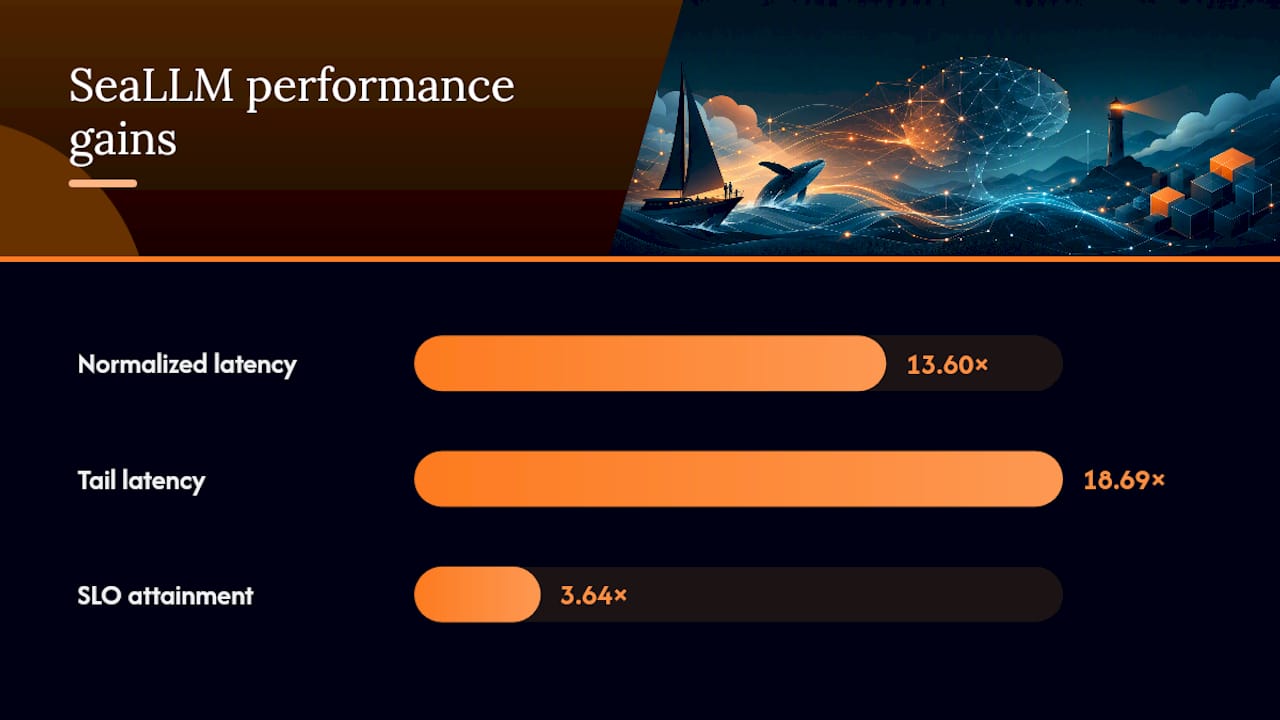
SeaLLM’s service-aware scheduling reported up to 13.60x normalized latency improvement, up to 18.69x tail latency improvement, and up to 3.64x SLO attainment improvement on a 32-GPU cluster using real production traces. These gains come from placement heuristics that co-locate models with complementary traffic patterns and from unified KV-cache sharing across model instances.

LLMProxy-style proxy patterns:

The LLMProxy architecture combines three components: a model adapter (routing), SmartContext (context compression), and a smart cache (semantic caching). Together, these components reduced costs by over 30% in deployment while maintaining quality. The lesson for enterprise teams: a proxy layer that handles all three functions is easier to govern, monitor, and update than three separate point solutions.

Implementation notes for a budget-aware control plane:

Instrument each pipeline phase with its own cost counter and quality signal (confidence score, human feedback, downstream task metric).
Profile cost-quality tradeoff curves for each phase using a representative workload sample before setting budget allocations.
Roll out budget constraints incrementally: start at 90% of unconstrained spend, validate quality metrics, then tighten in 10% steps.
Require a rollback trigger: if quality metrics drop more than 5% relative to baseline, automatically restore the previous budget allocation.

Teams managing multi-cloud AI governance alongside cost controls will find that budget-aware orchestration fits naturally into a policy-as-code governance model.

The organizational reality most teams skip

Cost optimization programs fail more often from organizational friction than from technical complexity. The routing logic is straightforward. Getting three teams to agree on a shared evaluation set is not.

The most common failure pattern: an engineering team implements a routing rule, it ships to production, and two weeks later a product manager notices that response quality on a specific feature has degraded. No one set up a quality regression alert. The optimization gets rolled back, and the team loses confidence in the whole program.

The fix is not more sophisticated tooling. It is a pre-agreed quality contract before any optimization ships. Define the minimum acceptable quality score for each feature, instrument it, and make it a blocking condition for any routing or caching change. That contract is what lets you move fast without breaking things.

When requesting resources from a FinOps team or CTO, the script that works is not “we want to optimize our LLM costs.” It is: “We are currently spending $X/month on LLM API calls. The engineering cost is Y hours. The quality risk is mitigated by this evaluation set and this rollback plan. We need approval to proceed and a shared dashboard so you can see the savings in real time.”

One candid warning: semantic cache invalidation is the most common source of silent quality degradation in production. When your underlying data changes (a product catalog update, a policy change, a new knowledge base version), cached responses become stale. Build cache invalidation triggers into your data pipeline, not as an afterthought.

Everythingcloud gives you continuous visibility into AI and LLM spend

Applying these tactics manually works, but it requires sustained engineering attention, cross-team coordination, and a monitoring stack that most organizations build piecemeal. Everythingcloud’s managed FinOps platform gives enterprise teams and MSPs real-time visibility into AI token consumption, automated anomaly detection, and budget enforcement across AWS, Azure, Google Cloud, and AI workloads, without building the observability layer from scratch.

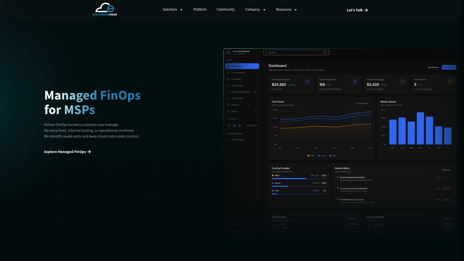
The platform continuously identifies optimization opportunities, automates cost-saving actions, and delivers expert recommendations every month. For MSPs, it is a turnkey “FinOps in a Box” that enables managed AI optimization services without building a proprietary solution. For enterprise IT and FinOps teams, it replaces the spreadsheet-and-alert patchwork with a governed, auditable cost control layer aligned to CIS and NIST standards.

If your team is past the point of manual tracking and ready for a continuous optimization loop, explore the Everythingcloud platform or speak with the team about a managed FinOps engagement.