
The fastest way to cut vector database bills is to change index type and stop loading the full dataset into memory. For many retrieval-augmented generation workloads, that combination alone can deliver 60 to 80% lower memory costs, run a canary now: swap to a compressed index on a representative subset and measure memory, recall, and latency before touching production.
TL;DR:
- Switching to compressed indices like IVF_SQ8 can reduce memory usage by about 70% with minimal recall loss, significantly lowering costs.
- Using memory-mapped storage or tiered storage can decrease resident memory to below 10%, reducing infrastructure expenses without major performance hits.
- Lowering vector dimensions from 1536 to 768 can cut storage and compute costs roughly in half while maintaining acceptable recall levels.
- Batch operations for ingestion and careful management of data lifecycle—such as compaction and TTL policies—can prevent unnecessary cost inflation.
- Continuous monitoring and automated remediation are key to maintaining savings, especially across multiple collections and changing workloads.
Table of Contents
- Where the money goes in a vector DB deployment
- Why memory dominates vector search costs
- Choose the right index and compression for your accuracy/cost needs
- Stop loading everything into RAM: MMap and tiered storage patterns
- Reduce embedding cost: dimension and model choices
- Ingestion, batching, and storage best practices (including S3 Vectors advice)
- Manage data lifecycle: compaction, TTL, and deletion
- Key metrics and dashboards to measure cost impact
- Priority roadmap: quick wins to medium to long-term actions
- How a managed FinOps approach operationalizes these tactics
- Risk-managed rollout matters more than clever tuning
- How EverythingCloud supports sustained vector database savings
- FAQ
- Sources
Where the money goes in a vector DB deployment
Before optimizing anything, you need to know what you are paying for. In a typical deployment, memory and compute account for roughly 85 to 90% of vector database infrastructure cost, with network and storage making up the remainder.
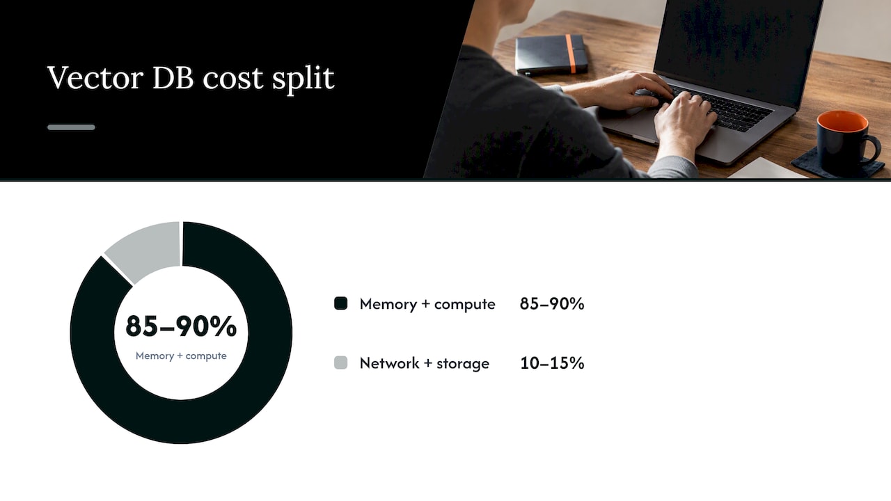
Memory and compute drive the majority of vector DB spend, often 85 to 90% of total infrastructure cost, according to Milvus’s cost optimization research. That single fact should reorder your entire optimization priority list.
Vendor pricing dimensions map directly onto these cost buckets:
- Vector dimensions stored drive memory footprint and often the billed unit itself.
- Storage volume determines object storage and backup charges, typically the smallest line item.
- Throughput (QPS) drives compute sizing and, indirectly, the number of nodes you provision.
- Network egress stays modest unless you return full vector payloads on every query.
Say a RAG workload stores 50 million vectors at 1536 dimensions in an uncompressed index. Memory alone could run into hundreds of gigabytes, pushing you onto the largest, most expensive instance tiers, while storage and network costs stay a fraction of that bill. The imbalance is the reason index and memory strategy outrank every other lever on this list.
Why memory dominates vector search costs
Vector search is not a simple lookup. Approximate nearest neighbor (ANN) indices scatter related vectors across memory in patterns that are inherently random-access, which means they are bandwidth-limited rather than compute-limited. Every query touches memory addresses that the CPU cannot predict, so prefetching helps far less than it does in sequential workloads.
Graph-based indices like HNSW compound this problem. Traversing the graph means following edges to neighbors that live in arbitrary memory locations, and each hop risks a cache miss. That translates directly into throughput and latency penalties once the index no longer fits comfortably in cache.
A few structural facts explain why this gets expensive fast:
- Dimension count multiplies memory linearly: doubling dimensions roughly doubles the footprint per vector.
- Graph-based indices add overhead for edge lists on top of the raw vectors themselves.
- Random-access patterns mean more RAM rarely gets you proportional throughput gains once you are bandwidth-bound.
- Larger indices increase the chance that hot paths spill out of CPU cache, adding latency even before memory pressure forces paging.
Understanding this is the reason compression and architecture-level changes, not just bigger instances, are the real fix. Research on compressed indices shows that reducing the memory footprint of stored vectors can cut bandwidth demand by up to roughly 8 times compared to uncompressed float32 storage, while preserving recall in billion-scale tests. That is the architecture-level lever worth testing before you simply add nodes.
Choose the right index and compression for your accuracy/cost needs
Index choice is the single biggest lever you control directly, and the trade-offs are well documented. Switching from HNSW or IVF_FLAT to a compressed variant like IVF_SQ8 can cut memory usage by roughly 70%, with a recall loss of only about 2 to 3%, which is acceptable for most RAG use cases.
Here is how the common options compare in practice:
- HNSW: fast and accurate but memory-hungry; best when latency budgets are tight and cost is secondary.
- IVF_FLAT: simpler than HNSW with similar memory demands; rarely the cheapest choice today.
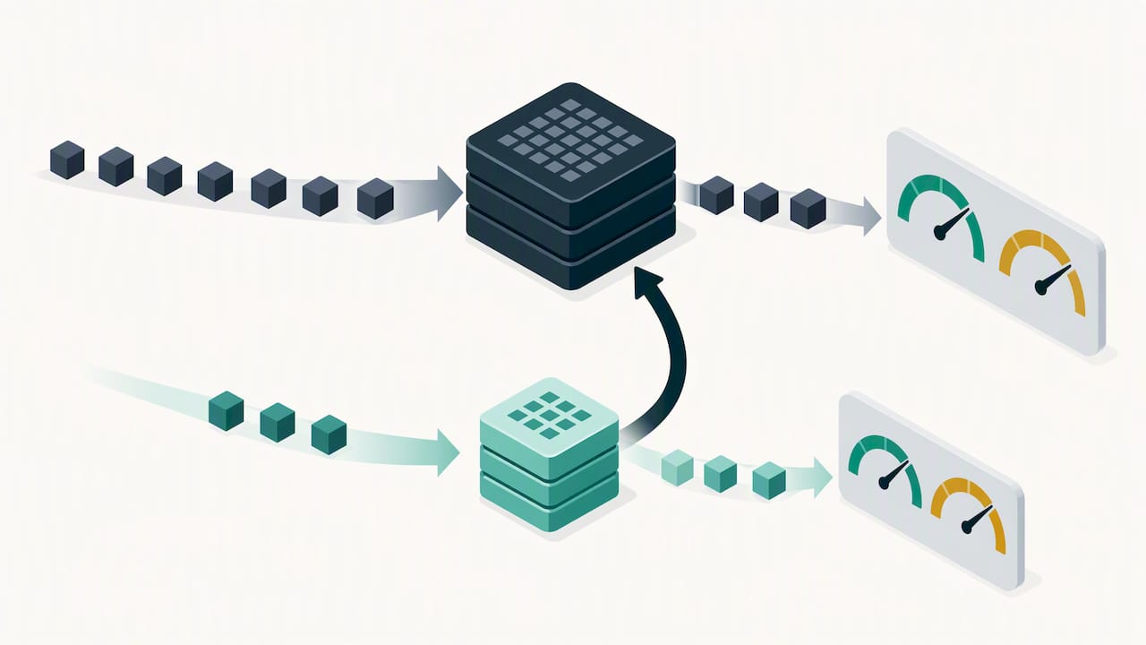
- IVF_SQ8: scalar quantization cuts memory roughly 4x versus uncompressed HNSW or FLAT with modest recall loss.
- IVF_PQ: product quantization compresses further still, trading more recall for smaller footprints on very large collections.
- DiskANN: built for datasets too large to fit in RAM, keeping most of the index on disk with strong recall at lower memory cost.
No single system wins every metric. A benchmark evaluation across seven vector database systems found that recall, throughput, latency, and resource use trade off differently depending on configuration and data distribution, which is why you test before you commit.
Measure P99 latency at each step, not just average latency.
Pro Tip: Keep the old index warm in a shadow deployment for at least one business cycle before decommissioning it, so rollback is a configuration change, not a rebuild.
Set rollback criteria before you start: if recall drops more than 3 to 5 percentage points below your target, or P99 latency exceeds your SLA, revert immediately and try the next compression tier down.
Stop loading everything into RAM: MMap and tiered storage patterns
The second-biggest lever is refusing to load your entire dataset into memory in the first place. MMap keeps the full dataset on local disk and maps it into virtual memory, letting the operating system page in only what queries actually touch. This can shrink resident memory to roughly 10 to 30% of full-load mode while keeping latency low for most query patterns.
Tiered storage goes further by putting object storage at the base tier and a local cache on top. Hit rate becomes the deciding variable here.
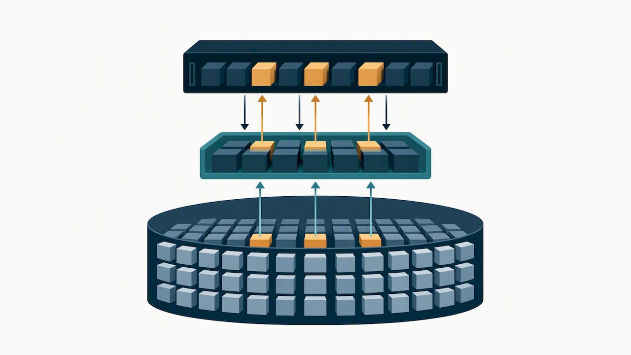
Tiered storage can push resident memory below 10% of full-load levels, depending on hot/cold data skew, per Milvus’s optimization guide, though cache misses carry a real latency penalty.
Before you flip this switch, work through the operational details:
- Size local disk to hold your full dataset comfortably if you choose MMap, not just the hot subset.
- Plan cache eviction policy deliberately; least-recently-used works for most access patterns but can thrash under bursty traffic.
- Budget for a latency penalty on cache misses, since a cold read from object storage is an order of magnitude slower than a memory hit.
- Monitor hit rate continuously, since a drop below your target signals you need either a bigger cache or better tiering rules.
These patterns pair well with each other: compress your index first, then decide how much of the compressed footprint actually needs to live in RAM.
Reduce embedding cost: dimension and model choices
Dimensionality multiplies both storage and compute cost in a straight line, which makes embedding model choice one of the highest-leverage decisions you make before a single vector is ever indexed. A workload storing vectors at 1536 dimensions runs roughly 4 times the cost of an equivalent workload at 384 dimensions, assuming similar index structure.
The practical question is whether a smaller model meets your accuracy bar:
- 1536-d models tend to sit at the high end of both cost and recall for general-purpose retrieval.
- 768-d models often recover most of the recall at roughly half the footprint.
- 384-d models can be competitive for narrower domains where the embedding space does not need to capture as much nuance.
Run the experiment properly: take a representative sample, re-embed it with the smaller model, and A/B test recall@K against your current production embeddings before committing to a full re-embed. A full re-embedding pipeline is higher-friction than an index swap, so stage it behind a feature flag and roll out by tenant or collection rather than all at once.
Pro Tip: Treat a small recall drop as acceptable only when it is measured against your actual downstream task, not just raw cosine similarity scores.
Ingestion, batching, and storage best practices (including S3 Vectors advice)
Inefficient ingestion quietly inflates your cost-per-operation long before you notice it in a monthly invoice. A few operational rules fix most of it:
- Batch upserts aggressively. AWS guidance for S3 Vectors recommends batching up to 500 vectors per API call to maximize throughput and avoid throttling.
- Split indexes by tenant when you serve multiple customers, so you can isolate cost per tenant and apply different compression tiers where usage patterns differ.
- Minimize payload size on the return path: fetch only IDs and scores from the vector store, then hydrate full documents from a cheaper storage layer only when needed.
These changes rarely require architectural rework, which makes them good first moves alongside your index canary. For teams running object storage underneath their vector layer, the same lifecycle and layout principles that apply to general S3 cost optimization carry over directly.
Manage data lifecycle: compaction, TTL, and deletion
Append-only designs accumulate tombstones, the markers left behind when a vector is logically deleted but not yet physically removed. Over time those tombstones bloat memory and force every query to scan past dead entries, which raises both cost and latency.
Compaction reclaims that wasted space by rewriting segments and dropping tombstoned data permanently. Schedule it during low-traffic windows and monitor job duration, since a compaction run that takes longer than expected usually signals an index that has grown past its planned size.
- Set TTL policies on collections with naturally expiring data, such as session embeddings or time-boxed document sets, so cleanup happens automatically.
- Use manual deletion only for exceptions, since automatic expiry removes an entire class of operational toil.
- Monitor compaction jobs for duration and resource spikes, and keep a rollback plan that pauses compaction if query latency degrades mid-run.
Key metrics and dashboards to measure cost impact
You cannot prove savings you are not measuring. A minimal metric set covers the full cost chain, from raw infrastructure signals to dollar impact.
| Metric | What it tells you |
|---|---|
| Resident memory (GiB) | Direct driver of instance size and monthly compute cost |
| Cache hit rate | Reveals whether tiered storage is saving money or just adding latency |
| Vector dimensions stored | Baseline for storage and compute scaling |
| QPS | Determines node count needed to meet latency SLAs |
| P99 latency | Guardrail against degrading user experience while optimizing cost |
| Recall@K | Guardrail against sacrificing quality for savings |
| Cost per million queries | The single number that ties every other metric to the bill |
Convert each infra metric into a dollar figure by tying it to your actual instance pricing: a 70% memory reduction on a given instance tier translates directly into a smaller instance class or fewer nodes, and that delta is your proof of ROI for the change.
- Set alert thresholds on cache hit rate dropping below your target, since that usually means your cache is undersized for current traffic.
- Alert on recall@K drifting below your acceptance floor after any index or embedding change.
- Trigger automated remediation, such as scaling a cache tier, when cost per million queries crosses a defined ceiling for more than one evaluation window.
Priority roadmap: quick wins to medium to long-term actions
Sequence matters. Start with reversible, fast-to-measure changes, then move to higher-friction work once you trust your measurement pipeline.
- Quick wins (days): swap index type on a canary collection, enable MMap or tiered storage, and fix obvious batching gaps in ingestion.
- Medium-term (weeks): run dimensionality experiments with a smaller embedding model, build adaptive tiering policies based on observed hot/cold skew, and put compaction on a schedule.
- Long-term (ongoing): formalize governance over index and embedding choices, stand up continuous monitoring against the metric set above, and automate remediation for cost anomalies.
Pro Tip: Never run more than one major change per collection at a time. When recall or latency shifts, you want to know exactly which lever caused it.
Each step carries its own rollback trigger: revert an index swap if recall or latency breaches your floor, pause a tiering rollout if cache hit rate stays low after a full day of representative traffic, and hold off on a dimension change if A/B recall testing shows a gap your downstream task cannot absorb.
How a managed FinOps approach operationalizes these tactics
Running this roadmap manually works for one collection. It breaks down across dozens of them, which is where continuous monitoring and automated remediation earn their keep instead of ad-hoc, one-time cleanups.
A managed FinOps engagement should give you:
- Continuous monitoring that flags memory, recall, and cost drift automatically rather than waiting for a quarterly review.
- Automated remediation actions, not just recommendations you still have to implement yourself.
- Invoice-level verification that ties every claimed saving back to an actual line item on your cloud bill.
- A clear baseline and playbook before any change is made, so you know exactly what “better” looks like.
Before signing with any partner, ask for a documented baseline, a written playbook mapped to your workloads, and proof that past savings were verified against real invoices rather than estimated.
Risk-managed rollout matters more than clever tuning
The biggest mistake we see is chasing the largest theoretical savings first instead of the safest one. Prioritize experiments that are reversible and measurable against real business KPIs, not just infrastructure metrics. Cost optimization that quietly regresses recall or latency is not optimization, it is a deferred outage. Stage every change behind a canary, watch it against your SLA, and only then expand.
— Dan
How EverythingCloud supports sustained vector database savings
Index swaps and tiering changes deliver real savings, but keeping them tuned as your data grows is where most teams run out of time. Our Continuous Cloud Optimization service pairs ongoing monitoring with automated remediation, so a cache hit rate drop or a memory spike gets flagged and acted on instead of discovered a month later on an invoice.
For MSPs building this as a service for clients, our Founding Partner Membership gives you a turnkey path to deliver managed FinOps without building the monitoring stack yourself. Either way, ask for a baseline analysis and a pilot scope before committing to a full rollout, and verify every claimed saving against your own invoices, not an estimate.
FAQ
Is the vector database outdated?
No. Vector databases remain the standard infrastructure for similarity search in RAG and recommendation systems, though benchmark research shows performance varies widely by system and configuration. The technology is maturing quickly, with compression and tiered storage reducing the cost concerns that once made it feel expensive.
How much does vector database cost?
Cost depends heavily on dataset size, dimension count, and index choice, since memory and compute typically account for 85 to 90% of total infrastructure cost. Vendor pricing models also vary: some bill by vector dimensions and storage, as described in Weaviate’s pricing structure, so comparing providers means comparing your actual workload against each model.
How to optimize a vector database?
Start with index compression and memory strategy, since switching to a compressed index like IVF_SQ8 combined with MMap or tiered storage can cut memory costs by 60 to 80% for many workloads. Pair that with batched ingestion, scheduled compaction, and continuous monitoring of recall and latency to protect quality while cutting cost.
What is replacing vector databases?
Nothing is broadly replacing vector databases today; instead, the field is converging on hybrid architectures that combine compressed indices, tiered storage, and smaller embedding models within existing systems. Research into compression methods like LVQ points toward evolution of the same core architecture rather than a wholesale replacement.
Sources
- How to Cut Vector Database Costs by Up to 80%: A Practical Milvus Optimization Guide
- Similarity search in the blink of an eye with compressed indices (LVQ)
- A Comprehensive Empirical Evaluation of Vector Database Systems for Approximate Nearest Neighbor Search
- S3 Vectors best practices – Amazon Simple Storage Service