
Cost variance analysis compares what you planned to spend with what you actually spent, then explains the gap. The core formula is simple: actual minus budget, or in project management, earned value minus actual cost. The hard part is the second step. A number alone tells you nothing until you know why it moved and whether anyone should act.
This guide covers the formulas you will meet in accounting and project management, a worked example for each, and the part most guides skip: how the method changes when the spend is cloud, SaaS and AI, where costs shift daily and a monthly review arrives too late.
TL;DR
- Cost variance is the gap between expected and actual cost. In earned value management, CV = EV − AC, and a negative result means over budget.
- Use percentages alongside dollars. A $5,000 miss means very different things on a $50,000 task and on a $5,000,000 program.
- Treat variance as a signal to understand, not a failure to punish. A spike can be healthy growth.
- For cloud, SaaS and AI spend, monthly analysis is too slow. A weekly checkpoint, backed by tagging and automated anomaly detection, catches drift before month-end.
- Finance and engineering need to read the same report, with every variance traceable to a service, account or tag.
Table of Contents
- What cost variance analysis actually measures
- The formulas you need
- A repeatable process
- Why the classic method strains on cloud, SaaS and AI spend
- Variance is a signal, not always waste
- Make finance and engineering read the same report
- Automating the investigation
- Applying it to SaaS and AI
- Our perspective: the variance report is only half the job
- Where EverythingCloud fits
- Common mistakes to avoid
- FAQ
- Sources
What cost variance analysis actually measures
A variance is, in the words of the PMBOK Guide as quoted by PMI, a quantifiable deviation from a known baseline or expected value. Cost variance analysis is the habit of measuring that deviation on a schedule, sorting it into causes, and deciding what to do.
Three things have to exist before the analysis means anything:
A baseline. This is a budget, a forecast or a standard cost. Without it you are only looking at spend, not variance.
An actual. This is the cost that really posted, ideally at the same level of detail as the baseline. If the budget is by department and the actuals are by vendor, you will spend your time reconciling instead of analyzing.
A owner for the explanation. Someone who understands the driver has to say what happened. In a factory that is a plant manager. In a cloud environment it is an engineering lead who knows why the instance count doubled.
The formulas you need
The phrase covers several calculations, depending on whether you work in project management, manufacturing accounting or budgeting. Here are the common ones.
Project cost variance (earned value)
Per the PMI explanation of earned value management, Cost Variance is EV minus AC. EV is the value of the work actually performed, and AC is the actual cost incurred. Zero means on budget, a positive number means under budget (favorable), and a negative number means over budget (unfavorable).
The companion measure is the Cost Performance Index: CPI = EV ÷ AC. A CPI of 1.0 is on target. Above 1.0 is efficient, and below 1.0 is not.
Example. A migration project has delivered work valued at $120,000 so far. It has cost $135,000. CV = 120,000 − 135,000 = −$15,000. CPI = 120,000 ÷ 135,000 = 0.89. Every dollar spent is buying about 89 cents of planned work.
Variance percentage
Absolute dollars hide scale. PMI literature on evaluating project performance notes that practitioners normalize with a percentage such as CV ÷ EV, so a $5,000 variance on a $50,000 task reads as far more serious than the same amount on a $5,000,000 project.
In the migration example above, CV% = −15,000 ÷ 120,000 = −12.5%. This is also the answer to the common question about what a 20% variance means: the actual figure differs from the baseline by one fifth of it. Whether that matters depends on your tolerance, which you should set in advance, for example by cost category.
Budget versus actual
For a department or cost center the general formula is actual minus budget. The sign convention flips depending on the line. Higher actual spend than budget is unfavorable for an expense. Higher actual revenue than budget is favorable. Agree on the convention before the first report goes out, or half your readers will misread the table.
Standard costing: price and usage variances
Manufacturing accounting splits a cost variance into two questions: did we pay the right price, and did we use the right quantity? As Lumen’s managerial accounting text/08%3A_Standard_Cost_Systems/8.03%3A_Calculations_for_Direct_Materials_and_Labor) lays it out:
- Material price variance: MPV = AQp × (SP − AP), where AQp is the actual quantity purchased, SP the standard price and AP the actual price. It measures purchasing efficiency.
- Material usage variance: MUV = SP × (SQA − AQu), where SQA is the standard quantity allowed and AQu the actual quantity used. A negative result signals more material consumed than the standard allows.
That answers another question people search: how is MUV calculated. Standard price times the difference between allowed and actual quantity.
Example. The standard allows 2 kg of resin per unit, at a standard price of $4 per kg. You made 1,000 units, so the allowed quantity is 2,000 kg, but you used 2,150 kg. MUV = $4 × (2,000 − 2,150) = −$600, unfavorable. If you also paid $4.20 per kg on 2,150 kg purchased, MPV = 2,150 × (4.00 − 4.20) = −$430, also unfavorable. The two variances point to different owners: production for usage, purchasing for price.
A repeatable process
The formulas are the easy part. A review that people trust follows the same steps each cycle.
- Fix the baseline and freeze it. Rewriting the budget mid-year to match reality erases the very signal you want. Keep the original and track re-forecasts separately.
- Pull actuals at the same granularity. Match the structure of the budget: project, department, product, account or tag.
- Calculate in dollars and percent. Flag anything beyond the tolerance you set in advance.
- Split price from volume. Ask whether you paid more per unit or consumed more units. The fix differs.
- Assign an explanation to a named owner. A variance with no owner repeats next month.
- Decide: act, accept or re-forecast. Some variances are a one-time event. Others change the forecast for the rest of the period.
- Feed the pattern into the forecast. PMI practitioners use these trends to project the Estimate at Completion, which is what turns variance data into a forecasting tool rather than a post-mortem.
The tone of the review matters as much as the arithmetic. The same PMI guidance frames variance analysis as diagnostic, not punitive. If teams expect blame, they will explain variances away instead of surfacing them.
Why the classic method strains on cloud, SaaS and AI spend
Standard costing assumes stable inputs. A resin price changes quarterly. A cloud bill can change by the hour. Three features of modern technology spend break the old rhythm.
Spend is usage-driven. Auto-scaling, a new data pipeline or an AI feature can multiply consumption without anyone approving a purchase order. The variance appears after the fact, in an invoice.
Price and usage interact. Commitments, reserved capacity and discounts mean an unfavorable variance may be a rate problem (coverage lapsed) or a volume problem (more workloads), and mixing them up sends the wrong team to investigate.
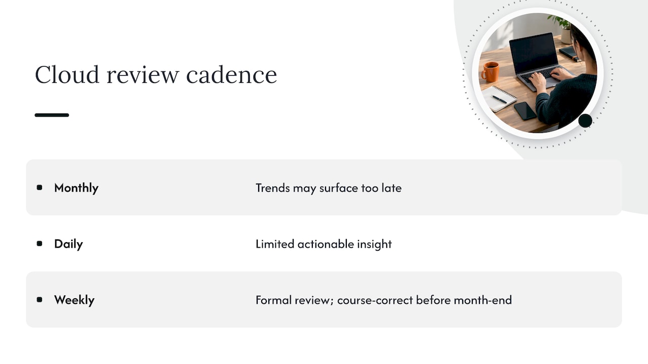
Monthly is too slow. AWS cloud financial management guidance from July 2026 says that monthly variance analysis may reveal trends too late for course correction, while daily tracking can produce limited actionable insight. Its answer is a weekly checkpoint that works as a formal review, with automated tooling supporting it. A weekly rhythm lets finance talk to technical teams before the month closes and keeps short-term noise from masking slow margin erosion.
This is the leak that compounds quietly. A 3% weekly drift looks like noise in any single report. Across a quarter it is a budget conversation nobody planned for.
Variance is a signal, not always waste
The most common mistake is treating every unfavorable variance as a problem to fix. The FinOps Foundation defines cloud cost anomalies as unpredicted variations in spend that deviate from historical patterns, and its framework stresses detecting, clarifying and managing them in a timely way. Notice the word clarify. A sharp rise after a successful feature launch is an unfavorable variance on paper and a good business outcome in practice.
To tell the two apart, you need allocation. If spend is mapped to a service, account, project or tag, you can see that the increase sits in the product that just launched and that revenue moved with it. If it is not mapped, the spike is a mystery and the default reaction is to cut. Our guide on reaching 90% allocation for cloud cost visibility goes into how enterprises get there.
A useful split is:
| Variance type | Typical cause | Right response |
|---|---|---|
| Value-driving consumption | Launch, growth, seasonal demand | Update the forecast, confirm unit economics |
| Waste | Idle resources, oversized instances, orphaned storage | Rightsize or remove, assign an owner |
| Rate variance | Lapsed commitment, lost discount, pricing change | Review coverage and renewals |
| Data or tagging issue | Untagged spend, misallocated shared cost | Fix allocation before drawing conclusions |
Make finance and engineering read the same report
Finance understands budgets and accruals. Engineering understands auto-scaling behavior and instance families. Neither side can interpret the other’s report. The AWS guidance on weekly checkpoints points to this gap and argues for moving from static spreadsheets to visibility where each variance links back to a specific service, principal or API action.
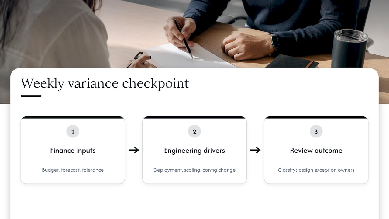
In practice that means the weekly checkpoint has two halves. Finance brings the budget, forecast and tolerance. Engineering brings the drivers, such as a deployment, a scaling event or a configuration change. The meeting ends with each variance labeled as expected, investigate or act, and an owner for every one that is not expected.
The same discipline applies to non-technical reporting. Whatever your function, the logic of regular, structured financial reviews is the same, as this overview of essential financial reports for business decisions shows for smaller companies. In the cloud, the difference is cadence and granularity: weekly, and down to the resource or tag.
If you are building the practice from scratch, our primer on what FinOps means for finance, engineering and leaders is a good place to align vocabulary first.
Automating the investigation
Manual root-cause work does not scale to thousands of line items. Native tooling is moving toward automated investigation. AWS documents an FinOps Agent preview that retrieves details of anomalies flagged by Cost Anomaly Detection, analyzes root causes ranked by cost impact and presents findings. The AWS weekly checkpoint article describes the same direction as conversational investigation, correlating cost changes with API activity in logs such as CloudTrail.
These tools shorten the time from alert to explanation. They do not decide whether a variance is acceptable, and they do not execute the fix. That judgment still needs the baseline, the tolerance and the owner described above.
Applying it to SaaS and AI
The same logic carries over. For SaaS, the baseline is the license count and contract value, and the usual variances are unused seats, overlapping tools and auto-renewals. Our overview of SaaS spend management for finance, IT and procurement covers who should own which part.
For AI, the volume driver is tokens and the price driver is model choice. A team that moves a workload to a larger model can create a price variance with no change in usage. Governance here means being able to see consumption by team and use case inside a single reporting cycle, which we describe in measuring AI cost governance.
For commitments on virtual machines, check whether variance comes from rate or usage before you buy more. The four FinOps levers for Azure VM cost optimization show what to verify first.
Our perspective: the variance report is only half the job
We work with MSPs and mid-market and enterprise teams, and the pattern we see is consistent. The variance report gets produced. The follow-through does not.
A dashboard that says spend is 14% over forecast is a diagnosis. The money comes back only when someone rightsizes the instance, adjusts the commitment or shuts down the idle environment. That is why we built EverythingCloud around automating the execution of optimization actions, not only listing recommendations. Savings outcomes are then checked against invoice-level billing, because the invoice is the number finance will actually pay.
For MSPs the stakes are sharper. When a customer’s cloud margin leaks, the provider often sees it last: commitments lapse, discounts are not passed through, and the pattern starts compounding before anyone reviews it. A weekly checkpoint, consistent allocation and automated actions across tenants are how you catch that without hiring a new team for each customer.
Our advice is to start small. Pick your three largest cost lines, set a tolerance for each, review weekly, and make sure every flagged variance has a named owner by the end of the meeting. Add automation once the process is stable.
— Dan
Where EverythingCloud fits
If you want the weekly checkpoint without staffing it yourself, our Managed FinOps service combines continuous monitoring with expert guidance, and Continuous Cloud Optimization covers AWS, Azure, Google Cloud, Microsoft 365 and AI workloads for enterprises. You can see how the pieces connect on The Platform page.
MSPs can launch these services under their own brand. The Founding Partner Membership is $500 per month.
Common mistakes to avoid
Rewriting the baseline. If the budget moves every time actuals miss, you have no variance to analyze.
Reporting dollars only. Add percentages so small and large items are comparable.
Reviewing monthly only. The AWS guidance argues for a weekly rhythm to avoid end-of-month surprises.
Ignoring tagging. Untagged spend turns every healthy spike into a suspicious one.
Stopping at the explanation. A documented variance with no action is the same variance next month.
FAQ
How do I calculate cost variance?
For projects, subtract actual cost from earned value: CV = EV − AC. A negative result means you are over budget. For a budget comparison, subtract the budget from actual spend and divide by the budget to get a percentage.
What does a 20% variance mean?
It means the actual figure is 20% above or below the baseline. Whether that is acceptable depends on the tolerance you set for that cost line, and on whether the cause is waste or value-driving growth. Review it with the owner before deciding.
How is MUV calculated?
Material usage variance equals the standard price times the difference between the standard quantity allowed and the actual quantity used. A negative result means more material was used than the standard permits.
How often should cloud cost variance be reviewed?
Monthly review alone tends to surface problems too late. AWS guidance published in July 2026 recommends adding a weekly checkpoint supported by automated tooling. Keep the monthly close for reporting and use the weekly review for action.
Sources
- PMI: Earned value management systems
- PMI: Earned value management standard
- PMI: The earned schedule
- Business LibreTexts: Calculations for direct materials and labor/08%3A_Standard_Cost_Systems/8.03%3A_Calculations_for_Direct_Materials_and_Labor)
- AWS: Improve your monthly cloud variance analysis with a weekly FinOps checkpoint
- FinOps Foundation: Anomaly management
- AWS FinOps Agent: Investigating cost anomalies